学习曲线（过拟合与欠拟合）

1. 多项式线性拟合

# 多项式
import numpy as np
x = 6*np.random.rand(100,1) -3
y = 2 + 0.5 * x ** 2 + x + np.random.rand(100, 1)

import matplotlib.pyplot as plt
plt.style.use('ggplot')
plt.scatter(x, y, s=2, c='red',alpha=0.7)
plt.show()

# 拟合多项式
from sklearn.preprocessing import PolynomialFeatures
poly_features = PolynomialFeatures(degree=2, include_bias=False)
x_ploy = poly_features.fit_transform(x)

## 用将特征装换为 x的一次和x的二次
from sklearn.linear_model import LinearRegression
lr = LinearRegression()
lr.fit(x_ploy, y)
lr.intercept_, lr.coef_

# 图示
y_1 = lr.predict(x_ploy)
plt.scatter(x, y, s=2, c='steelblue',alpha=0.7)
plt.scatter(x, y_1, c='red', s=3, alpha=0.6)
plt.show()

2、 学习曲线

画出模型在训练集上的表现，同时画出训练规模自变量的训练集函数。
为了得到图像，需要在训练集的不同规模子集上进行多次训练

欠拟合

def plot_learning_curves(model, x, y):
    x_train, x_test, y_train, y_test = train_test_split(x, y, test_size = 0.2)
    train_errors, test_errors = [], []
    for m in range(1, len(x_train)):
        model.fit(x_train[:m], y_train[:m])
        y_train_pre = model.predict(x_train[:m])
        y_test_pre = model.predict(x_test)
        train_errors.append(mean_squared_error(y_train_pre, y_train[:m]))
        test_errors.append(mean_squared_error(y_test_pre, y_test))

    plt.plot(np.sqrt(train_errors),'r-+', lw=2, label='train')
    plt.plot(np.sqrt(test_errors),'b-', lw=2, label='test')
    plt.legend(loc = 'upper right')
    plt.ylim(0,3)
    plt.show()


lr = LinearRegression()
plot_learning_curves(lr, x, y)

当加入一些新的样本的时候，训练集的拟合程度变的难以接受：
原因一：数据中含有噪声，
原因二：数据根本不是线性的
随着着数据规模的增大，误差也会一直增大，直到达到高原地带并趋于稳定，
在之后，继续加入新的样本，模型的平均误差不会变得更好或者更差

过拟合

from sklearn.pipeline import Pipeline
ploynomial_regression = Pipeline((
    ('poly_reg', PolynomialFeatures(degree=10, include_bias=False)), # 高阶多项拟合
    ('lr', LinearRegression()),
))
plot_learning_curves(ploynomial_regression, x, y)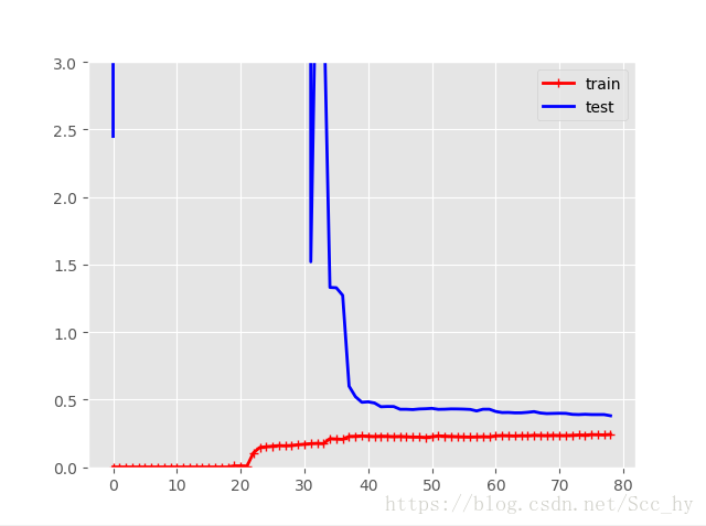

在训练集上，误差要比线性回归模型低的多。
图中的两条曲线之间有间隔，这意味模型在训练集上的表现要比验证集上好的多，这也是模型过拟合的显著特点。当然，如果你使用了更大的训练数据，这两条曲线最后会非常的接近。

3、一个模型的泛化误差由三个不同误差的和决定：

• 偏差：泛化误差的这部分误差是由于错误的假设决定的。例如实际是一个二次模型，你却假设了一个线性模型。一个高偏差的模型最容易出现欠拟合。
• 方差：这部分误差是由于模型对训练数据的微小变化较为敏感，一个多自由度的模型更容易有高的方差（例如一个高阶多项式模型），因此会导致模型过拟合。
• 不可约误差：这部分误差是由于数据本身的噪声决定的。降低这部分误差的唯一方法就是进行数据清洗（例如：修复数据源，修复坏的传感器，识别和剔除异常值）。