深度学习-神经网络基础 吴恩达第一课第二周作业1(Python Basics with Numpy)
1 - Building basic functions with numpy
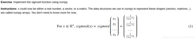
1.1 - sigmoid function, np.exp()
# GRADED FUNCTION: sigmoid

import numpy as np # this means you can access numpy functions by writing np.function() instead of numpy.function()

def sigmoid(x):
    """
    Compute the sigmoid of x

    Arguments:
    x -- A scalar or numpy array of any size

    Return:
    s -- sigmoid(x)
    """

    ### START CODE HERE ### (≈ 1 line of code)
    s = 1.0/(1.0 + np.exp(-x))
    ### END CODE HERE ###

    return s

x = np.array([1, 2, 3])
sigmoid(x)
1.2 - Sigmoid gradient

# GRADED FUNCTION: sigmoid_derivative

def sigmoid_derivative(x):
    """
    Compute the gradient (also called the slope or derivative) of the sigmoid function with respect to its input x.
    You can store the output of the sigmoid function into variables and then use it to calculate the gradient.

    Arguments:
    x -- A scalar or numpy array

    Return:
    ds -- Your computed gradient.
    """

    ### START CODE HERE ### (≈ 2 lines of code)
    s = sigmoid(x)
    ds = s * (1 - s)
    ### END CODE HERE ###

    return ds

x = np.array([1, 2, 3])
print ("sigmoid_derivative(x) = " + str(sigmoid_derivative(x)))
1.3 - Reshaping arrays
- X.shape is used to get the shape (dimension) of a matrix/vector X.
- X.reshape(...) is used to reshape X into some other dimension.
# GRADED FUNCTION: image2vector
def image2vector(image):
    """
    Argument:
    image -- a numpy array of shape (length, height, depth)

    Returns:
    v -- a vector of shape (length*height*depth, 1)
    """

    ### START CODE HERE ### (≈ 1 line of code)
    v = image.reshape( (image.shape[0] * image.shape[1] * image.shape[2], 1))
    ### END CODE HERE ###

    return v

# This is a 3 by 3 by 2 array, typically images will be (num_px_x, num_px_y,3) where 3 represents the RGB values
image = np.array([[[ 0.67826139,  0.29380381],
        [ 0.90714982,  0.52835647],
        [ 0.4215251 ,  0.45017551]],

       [[ 0.92814219,  0.96677647],
        [ 0.85304703,  0.52351845],
        [ 0.19981397,  0.27417313]],

       [[ 0.60659855,  0.00533165],
        [ 0.10820313,  0.49978937],
        [ 0.34144279,  0.94630077]]])

print ("image2vector(image) = " + str(image2vector(image)))
1.4 - Normalizing rows

# GRADED FUNCTION: normalizeRows

def normalizeRows(x):
    """
    Implement a function that normalizes each row of the matrix x (to have unit length).

    Argument:
    x -- A numpy matrix of shape (n, m)

    Returns:
    x -- The normalized (by row) numpy matrix. You are allowed to modify x.
    """

    ### START CODE HERE ### (≈ 2 lines of code)
    # Compute x_norm as the norm 2 of x. Use np.linalg.norm(..., ord = 2, axis = ..., keepdims = True)
    x_norm = np.linalg.norm(x, ord=2, axis=1, keepdims=True)

    # Divide x by its norm.
    x = x/x_norm
    ### END CODE HERE ###

    return x

x = np.array([
    [0, 3, 4],
    [1, 6, 4]])
print("normalizeRows(x) = " + str(normalizeRows(x)))
1.5 - Broadcasting and the softmax function

# GRADED FUNCTION: softmax

def softmax(x):
    """Calculates the softmax for each row of the input x.

    Your code should work for a row vector and also for matrices of shape (n, m).

    Argument:
    x -- A numpy matrix of shape (n,m)

    Returns:
    s -- A numpy matrix equal to the softmax of x, of shape (n,m)
    """

    ### START CODE HERE ### (≈ 3 lines of code)
    # Apply exp() element-wise to x. Use np.exp(...).
    x_exp = np.exp(x)

    # Create a vector x_sum that sums each row of x_exp. Use np.sum(..., axis = 1, keepdims = True).
    x_sum = np.sum(x_exp, axis=1, keepdims = True)

    # Compute softmax(x) by dividing x_exp by x_sum. It should automatically use numpy broadcasting.
    s = x_exp/x_sum

    ### END CODE HERE ###

    return s

x = np.array([
    [9, 2, 5, 0, 0],
    [7, 5, 0, 0 ,0]])
print("softmax(x) = " + str(softmax(x)))
2) Vectorization
In deep learning, you deal with very large datasets. Hence, a non-computationally-optimal function can become a huge bottleneck in your algorithm and can result in a model that takes ages to run. To make sure that your code is computationally efficient, you will use vectorization. For example, try to tell the difference between the following implementations of the dot/outer/elementwise product.
import time

x1 = [9, 2, 5, 0, 0, 7, 5, 0, 0, 0, 9, 2, 5, 0, 0]
x2 = [9, 2, 2, 9, 0, 9, 2, 5, 0, 0, 9, 2, 5, 0, 0]

### CLASSIC DOT PRODUCT OF VECTORS IMPLEMENTATION ###
tic = time.process_time()
dot = 0
for i in range(len(x1)):
    dot+= x1[i]*x2[i]
toc = time.process_time()
print ("dot = " + str(dot) + "\n ----- Computation time = " + str(1000*(toc - tic)) + "ms")

### CLASSIC OUTER PRODUCT IMPLEMENTATION ###
tic = time.process_time()
outer = np.zeros((len(x1),len(x2))) # we create a len(x1)*len(x2) matrix with only zeros
for i in range(len(x1)):
    for j in range(len(x2)):
        outer[i,j] = x1[i]*x2[j]
toc = time.process_time()
print ("outer = " + str(outer) + "\n ----- Computation time = " + str(1000*(toc - tic)) + "ms")

### CLASSIC ELEMENTWISE IMPLEMENTATION ###
tic = time.process_time()
mul = np.zeros(len(x1))
for i in range(len(x1)):
    mul[i] = x1[i]*x2[i]
toc = time.process_time()
print ("elementwise multiplication = " + str(mul) + "\n ----- Computation time = " + str(1000*(toc - tic)) + "ms")

### CLASSIC GENERAL DOT PRODUCT IMPLEMENTATION ###
W = np.random.rand(3,len(x1)) # Random 3*len(x1) numpy array
tic = time.process_time()
gdot = np.zeros(W.shape[0])
for i in range(W.shape[0]):
    for j in range(len(x1)):
        gdot[i] += W[i,j]*x1[j]
toc = time.process_time()
print ("gdot = " + str(gdot) + "\n ----- Computation time = " + str(1000*(toc - tic)) + "ms")
x1 = [9, 2, 5, 0, 0, 7, 5, 0, 0, 0, 9, 2, 5, 0, 0]
x2 = [9, 2, 2, 9, 0, 9, 2, 5, 0, 0, 9, 2, 5, 0, 0]
### VECTORIZED DOT PRODUCT OF VECTORS ###
tic = time.process_time()
dot = np.dot(x1,x2)
toc = time.process_time()
print ("dot = " + str(dot) + "\n ----- Computation time = " + str(1000*(toc - tic)) + "ms")
### VECTORIZED OUTER PRODUCT ###
tic = time.process_time()
outer = np.outer(x1,x2)
toc = time.process_time()
print ("outer = " + str(outer) + "\n ----- Computation time = " + str(1000*(toc - tic)) + "ms")
### VECTORIZED ELEMENTWISE MULTIPLICATION ###
tic = time.process_time()
mul = np.multiply(x1,x2)
toc = time.process_time()
print ("elementwise multiplication = " + str(mul) + "\n ----- Computation time = " + str(1000*(toc - tic)) + "ms")
### VECTORIZED GENERAL DOT PRODUCT ###
tic = time.process_time()
dot = np.dot(W,x1)
toc = time.process_time()
print ("gdot = " + str(dot) + "\n ----- Computation time = " + str(1000*(toc - tic)) + "ms")2.1 Implement the L1 and L2 loss functions

# GRADED FUNCTION: L1

def L1(yhat, y):
    """
    Arguments:
    yhat -- vector of size m (predicted labels)
    y -- vector of size m (true labels)

    Returns:
    loss -- the value of the L1 loss function defined above
    """

    ### START CODE HERE ### (≈ 1 line of code)
    loss = np.sum( np.abs(yhat - y))
    ### END CODE HERE ###

    return loss

yhat = np.array([.9, 0.2, 0.1, .4, .9])
y = np.array([1, 0, 0, 1, 1])
print("L1 = " + str(L1(yhat,y)))
# GRADED FUNCTION: L2

def L2(yhat, y):
    """
    Arguments:
    yhat -- vector of size m (predicted labels)
    y -- vector of size m (true labels)

    Returns:
    loss -- the value of the L2 loss function defined above
    """

    ### START CODE HERE ### (≈ 1 line of code)
    loss = np.dot( (yhat - y), (yhat - y))
    ### END CODE HERE ###

    return loss

yhat = np.array([.9, 0.2, 0.1, .4, .9])
y = np.array([1, 0, 0, 1, 1])
print("L2 = " + str(L2(yhat,y)))